How To Lock Cells In Google Sheets Formula
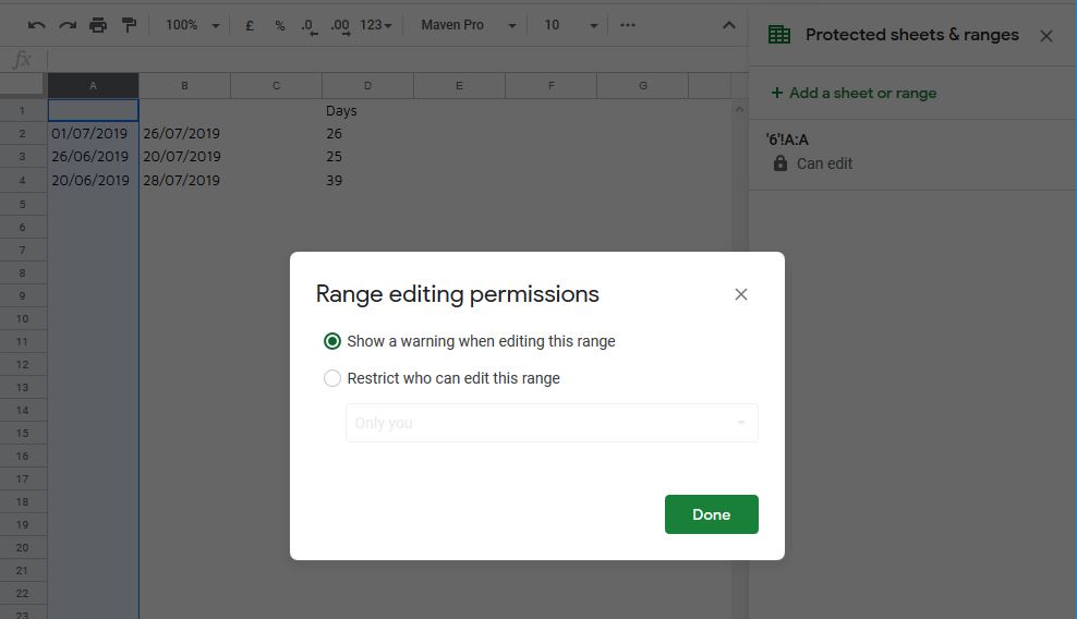
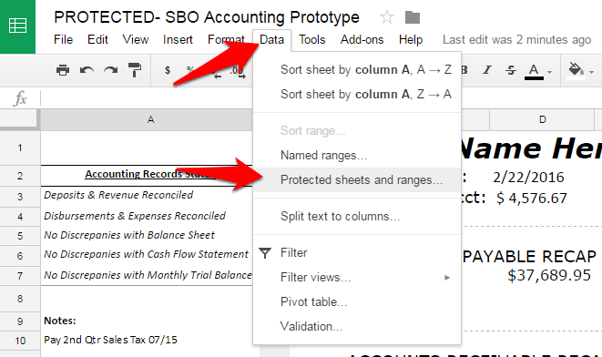
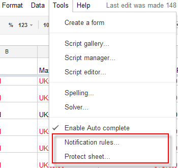
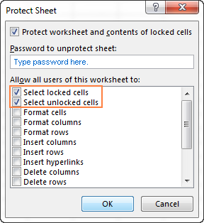
Then go to the data protected sheets and ranges menu to start protecting these cells.
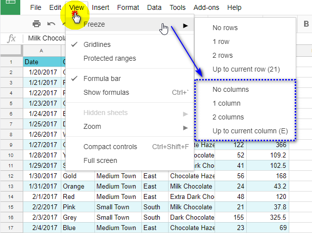
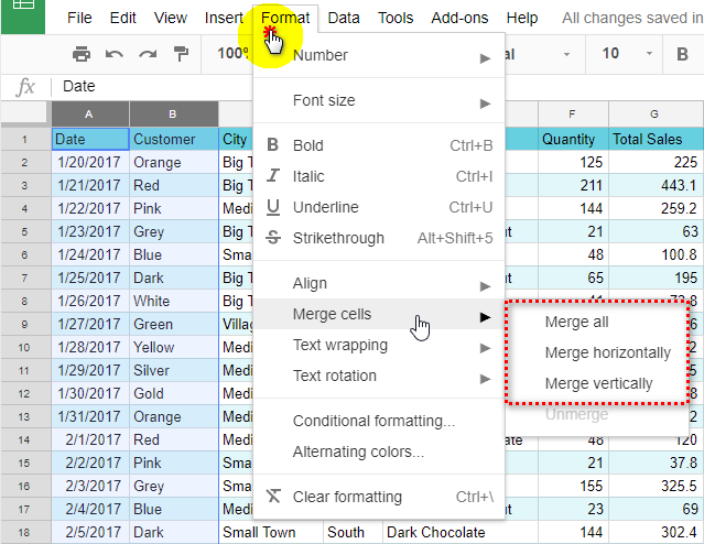
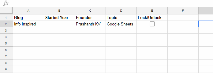
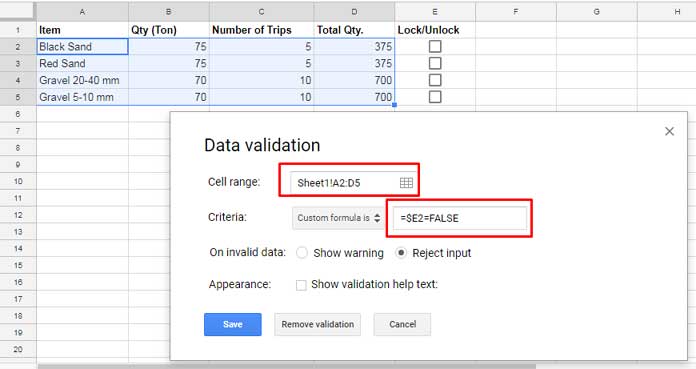
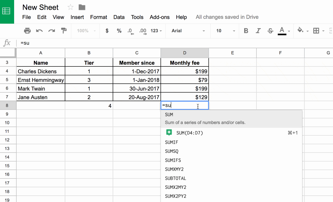
How to lock cells in google sheets formula. Use the data protected sheets and ranges menu option to start protecting specific cells in a google sheet. See the example below for the menu option. Sometimes its only a certain set of cells that you want to lock up in a spreadsheet. If you only need to lock one or more formula cells in a spreadsheet follow these instructions.
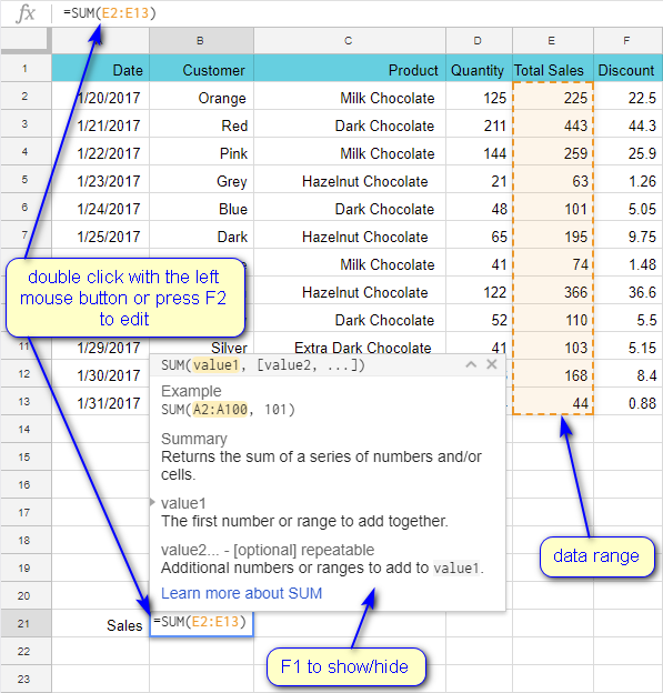
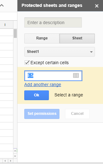
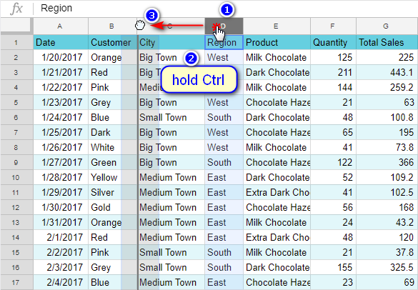
With the cells selected open the data menu and then click protect sheets and ranges the protected sheets and ranges pane appears on the right. Fire up your browser open a google sheet that has cells you want to protect and then select the cells. Open the google docs spreadsheet which you are going to collaboratively work on. Continue with the rest of your formula.
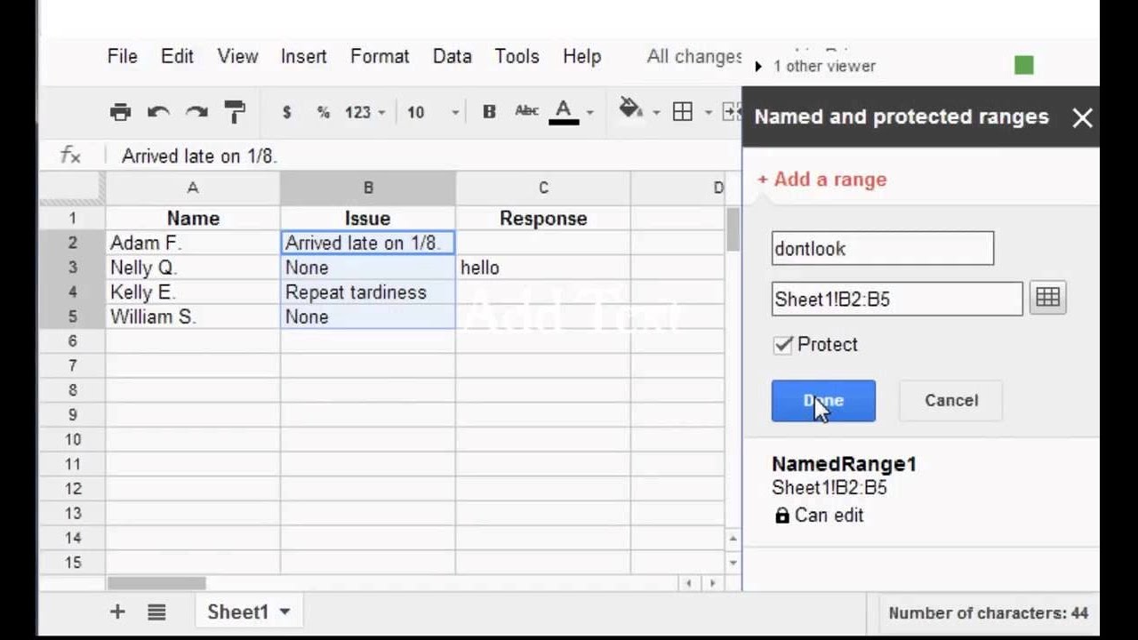
In the dialog box which opens up on the right you can give your named range a nickname keep it short. First up start off by highlighting a cell or range of cells that you want to protect. In those cases heres how to lock specific cells in google sheets. Protect cell ranges and lock them down.
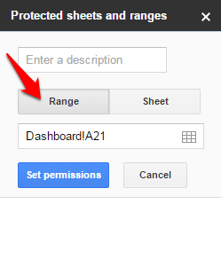
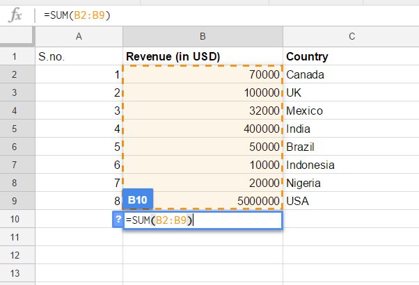
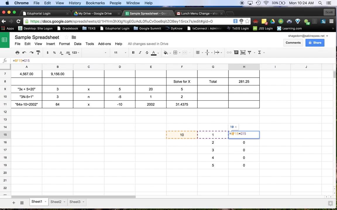
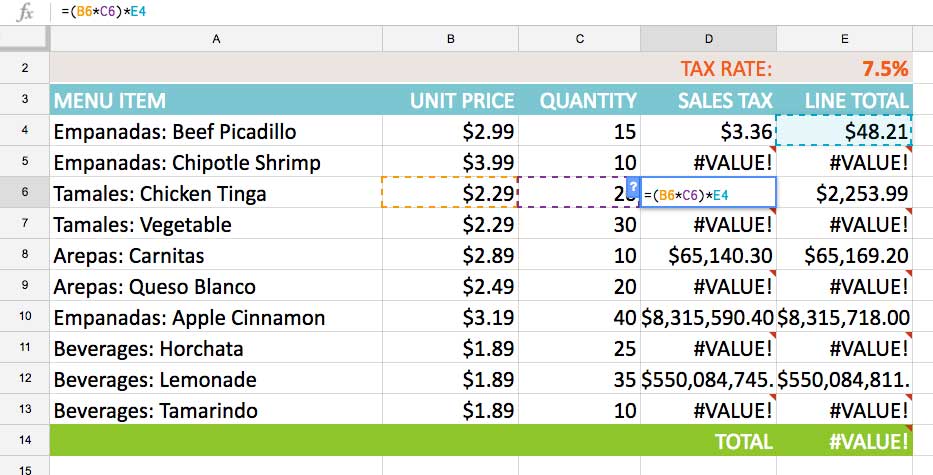
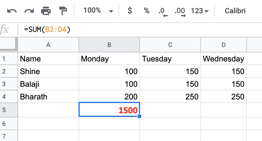
Open the protected sheets and ranges dialogue box select the range tab then click the select data range option shown in the screenshot below left click the mouse and drag the cursor over the formula.

Google Sheets Lock Rows Lock Columns Lock Ranges So Much

How To Lock A Formula In Google Sheets
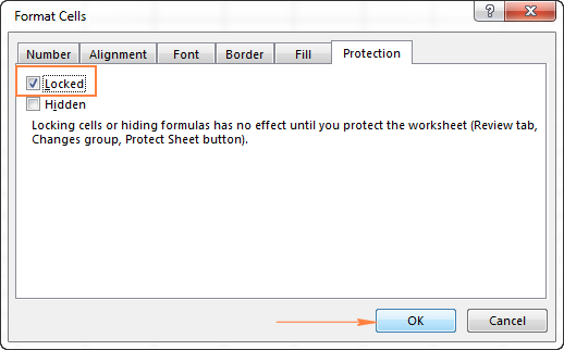
How To Lock And Hide Formulas In Excel

How To Lock A Formula In Google Sheets
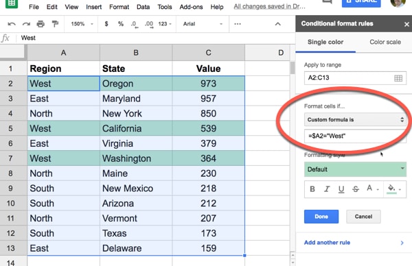
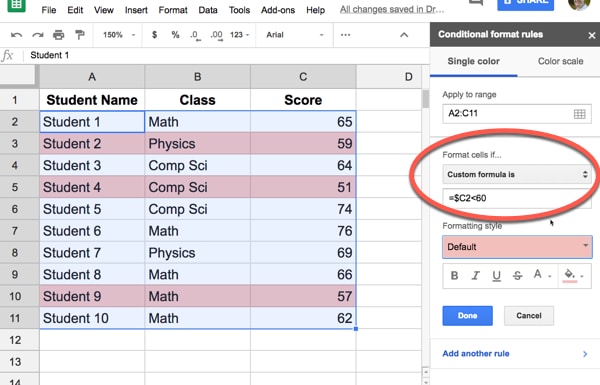
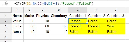
How To Apply Conditional Formatting Across An Entire Row In Google


:max_bytes(150000):strip_icc()/001-show-hide-formulas-in-excel-and-google-spreadsheets-3123884-91019d3fd12c4e7ab92558328e9788a9.jpg)


:max_bytes(150000):strip_icc()/003-show-hide-formulas-in-excel-and-google-spreadsheets-3123884-5fe1e7b82fc64d32bc032c0d3661fca5.jpg)